Lock column headers in excel 2013. How to Freeze and Unfreeze Rows and Columns in Excel 2019-02-12
Freeze panes to lock rows and columns
A thick line also initially separates the rows where there are hidden rows. Hello Erin, I'm sorry, but there is no way to change the standard headings in Excel. If you want, you can use our. Lock and protect selected cells from viewing by encrypting 1. When this is done, the headers for the rows and columns remain on the screen as the user scrolls horizontally or vertically through the workbook.
Freeze panes to lock rows and columns

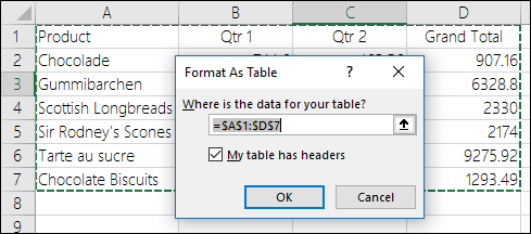
Right-click on one of the row headers selected and select Hide from the popup menu. The top row in our example sheet is a header that might be nice to keep in view as you scroll down. Add a Header Row Enter the column headings for your data across the top row of the spreadsheet, if necessary. Worksheets can be rearranged if needed. Notice that there are a bunch of rows at the top before the actual header we might want to freeze—the row with the days of the week listed. Also, you only select entire rows or columns to repeat.
How to Lock Cells in Excel (with Pictures)

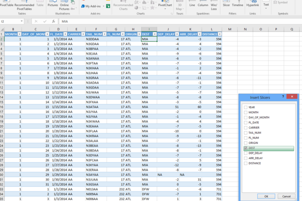
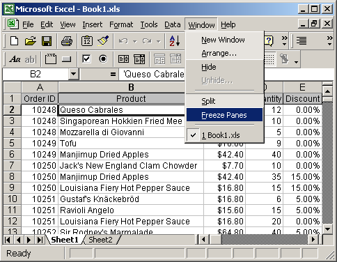
Here, the worksheet is scrolled so that the data in columns M through P appear after the data in column A. A black line displays to indicate the frozen rows and columns. This issue in Excel doesn't have a simple solution, but there is a workaround you can use. In our example, we want to freeze rows 1 and 2, so we'll select row 3. Changing Title Name Definitions If you change a worksheet so that the row or column titles are in different locations, you can edit or delete the existing names. Therefore, as you Enter or Analyze the data, the Month and Location remain visible if you scrolled down or to the right. If you had faced this previously, any update on the same will be a ppreciated.
The Simplest Way to Add a Header Row in Excel
For instance, to lock the first 2 rows and 2 columns, you select cell C3; to fix 3 rows and 3 columns, select cell D4 etc. Notice that rows three and four in the following image are hidden as well. Just select the cell to the right of the column you want to keep visible, and right below the row before clicking the button. Hi, Thanks for your reply, I used above code. Because just like , one day you may find out it simply doesn't work for you. As you move through your large spreadsheet, the headings disappear.
How to Hide and Unhide Rows and Columns in Excel 2013
The save will not stick? If this doesn't help, could you please specify what version of Excel you have and what steps you follow? For example, you can choose to open a new window for your workbook or split a worksheet into separate panes. Regards, AnandaBalan My problem, also. Below you will find the steps for both scenarios. If yes, use the Unfreeze Panes feature. In our example, the headings are in Column A or the First Column; therefore, the Freeze First Column feature is used to lock the headings in this worksheet. A little darker and thicker border to the right of column A means that the left-most column in the table is frozen.
Excel 2013: Freezing Panes and View Options

That way, I can see the first row and first column at all times even when I scroll. For example, if you select row 4 while the first 3 rows are out of view not hidden, just above the scroll and click Freeze Panes, what would you expect? They are created by the author or user of the workbook so that any subsequent use of the workbook does not require that you or anyone else need to define them. You can move the box to any location you prefer. Fortunately, Excel includes several tools that make it easier to view content from different parts of your workbook at the same time, such as the ability to freeze panes and split your worksheet Optional: Download our. Recommendation: Press Ctrl + Home prior to using the Freeze Top Row feature. Without the Column headings being visible, it becomes really difficult to enter new data in to proper Columns or to review and compare the existing data.
Keep Row and Column Headings Visible in Excel

M53 would be a range with column titles only with the bottom right cell of the range in cell M53. To create this article, volunteer authors worked to edit and improve it over time. Can I attach my excel example? I am using Excel 2016 for Mac. Use this little handy feature to have the headers visible when you scroll and always know what figures you are looking at. However, you can tell where the rows are hidden by the missing row headers. Though, you would still be able to get to the cells in a hidden frozen row using the arrow keys. To select the row, just click the number to the left of the row.
MS Excel 2013: Freeze first row and first column

The faint line that appears between Column A and B shows that the first column is frozen. You can try something like this, although you may want to test it in various browsers in case the column heading alignment is off. You can edit these names by selecting the cell. Whenever you lock rows or columns, the Freeze Panes option turns into Unfreeze Panes for you to quickly unlock the row or column. Answer: Traditionally, column headings are represented by letters such as A, B, C, D. Note that a thick gray line will always show you where the freeze point is. Now the rows above the selected Cell will remain frozen when you scroll down and also the Columns to the left of the selected Cell will also remain frozen when you scroll to the side.
Freeze panes to lock rows and columns
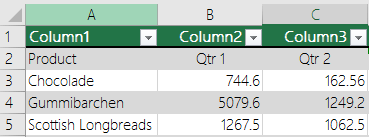
If your spreadsheet shows the columns as numbers, you can change the headings back to letters with a few easy steps. Excel for Office 365 Excel 2019 Excel 2016 Excel 2013 Excel 2010 Excel 2007 Excel Online To keep an area of a worksheet visible while you scroll to another area of the worksheet, go to the View tab, where you can Freeze Panes to lock specific rows and columns in place, or you can Split panes to create separate windows of the same worksheet. How to Modify Freeze Panes or Unlock the Row or Column: Do you want to modify what Rows or Columns are frozen? The column headings will be letters and the row headings will be numbers. When you perform other actions on the spreadsheet, this thick line will disappear. He is currently pursuing his master's degree in journalism at Clarion University. Is there any way we can apply some client side script to freeze column headers to listview webpart while scrolling down? The good news is that you can easily fix that inconvenience by freezing panes in Excel. See what happens when you scroll the worksheet to the right.