Lock cells in excel. How to Lock Cells in Excel (with Pictures) 2019-04-21
How to Protect Cell Data in Excel 2010

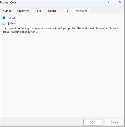
The procedure of adding them is given below. The following procedure gives you the answer. Step 3: Right-click one of the selected cells, then click Format Cells. By default, Excel locks all the cells in a protected worksheet and then you can specify which cells you want to unlock for editing if any. Users cannot apply or remove AutoFilters on a protected worksheet, regardless of this setting. You can select non-adjacent cells or ranges by holding the Ctrl key, or the entire sheet by pressing the Ctrl + A shortcut. This tutorial shows how to hide formulas in Excel so they do not show up in the formula bar.
How to Lock & Unlock an Excel Spreadsheet
Alternatively, under the Home tab, click on the expansion icon next to Alignment, and in the Format Cells window go to the Protection tab. More information about the worksheet elements Clear this check box To prevent users from Select locked cells Moving the pointer to cells for which the Locked check box is selected on the Protection tab of the Format Cells dialog box. If you want to undo the shared option, click on top of the excel file where Protect and Share Workbook Legacy is written. Tick on the Sharing with track changes and give a password. Format columns Using any of the column formatting commands, including changing column width or hiding columns Home tab, Cells group, Format button.
How to lock and hide formulas in Excel

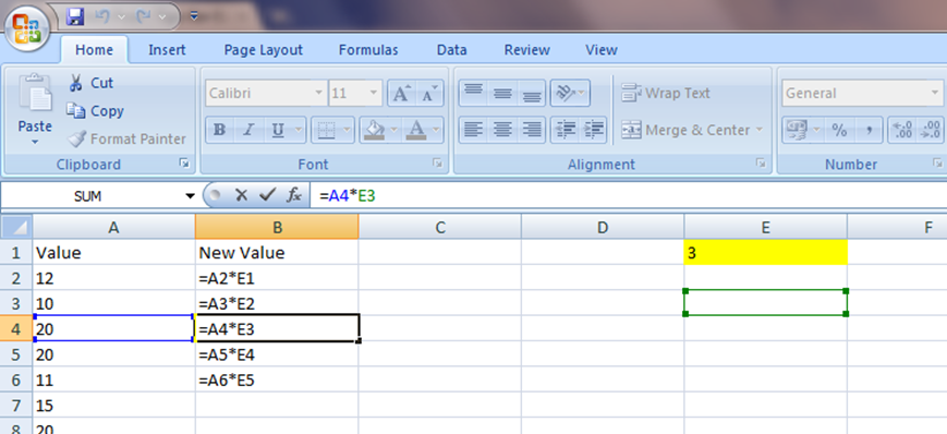
Luckily, Microsoft Excel makes it fairly simple to hide and lock all or selected formulas in a worksheet, and further on in this tutorial we will show the detailed steps. It returns a Boolean value based on whether the cell or range has a formula. Sharing locked Workbook- Improving Excel Security: When you have locked or protected the sheet, sharing has to be enabled. So now Select whole table as like above picture. Note: if you also check the Hidden check box, users cannot see the formula in the formula bar when they select cell A2. Edit scenarios Viewing scenarios that you have hidden, making changes to scenarios that you have prevented changes to, and deleting these scenarios. A simple loop can be used to detect cells in a given range that contain formula.
How to lock and protect selected cells in Excel?

In the resulting dialog box, you have an option of giving Password as well as tracking changes. Users can change the values in the changing cells, if the cells are not protected, and add new scenarios. This command freezes the left column of your spreadsheet, regardless which cell you've selected. Step 5: Click the Home tab at the top of the window. Before you start: by default, all cells are locked.
How to Lock a Cell in Excel 2010

To make sure of this, select any cell with a formula, and look at the formula bar, the formula will still be there. If you want to freeze more than just one row or one column, click the cell in the spreadsheet that's just to the right of the last column you want to freeze and just below the last row you want to freeze. How to Lock Specific Cells in a Worksheet There would be times or requirements when the pre-user wants that only certain cells should be available for the users to edit or format, while the other cells should store that data permanently, and should not be made available to edit, which may lead to erroneous results or impacts. To do this, use Excel's Freeze Panes function. Step 5: In the Go To Special dialog box, check the radio button.
Learn Excel Security
Users entering data into the wrong cells or changing existing formulas can make data collection a tedious process. The Select Locked Cells and Select Unlocked Cells check boxes are selected by default, but you can deselect either or both of these options if you prefer. For example, when sending some reports outside your organization, you may want the recipients to see the final values, but you don't want them to know how those values are calculated, let along making any changes to your formulas. About the Author Steven Melendez is an independent journalist with a background in technology and business. Don't need any special skills, save two hours every day! Chart sheet elements Select this check box To prevent users from Contents Making changes to items that are part of the chart, such as data series, axes, and legends. How to freeze rows and columns in excel Freezing is not a lock option but when there is a big data that you are analyzing and you want to work in a specific location of your excel file freezing the data is an effective way of doing that.
How to Lock & Unlock an Excel Spreadsheet

Tips: When you want to unprotect it again, just simply select Review tab, then click and use your given password. A warning box saying This action will save the workbook. Right click, and then click Format Cells. The following steps will guide you to unlock all cells in current firstly, lock required cells and ranges, and then protect current worksheet. Click either Freeze First Column or Freeze First Row to freeze the appropriate section of your data.
How to Lock a Cell in Excel 2010

How would you like to do? This tip will not allow viewing hidden columns, adding, deleting or moving worksheets and showing source data for pivot tables thereby improving excel security. Users cannot apply or remove AutoFilters on a protected worksheet, regardless of this setting. In doing so, you can choose whether users are allowed to select or edit a specific cell or a large array of cells, insert or delete rows or columns, allow conditional formatting, sort specific content in a sheet or variety of other options, that can only be applied to cells not locked or cells that are available for editing. Otherwise, the cell becomes or remains unlocked. However, you can check additional options on this window if you also want to allow them to make other changes. You can also click the Collapse Dialog button, select the range in the worksheet, and then click the Collapse Dialog button again to return to the dialog box.