Excel top 10 values. Excel formula: Sum top n values with criteria 2019-03-30
Extracting the top 5 maximum values in excel
Here is another good explaination of the Large formula. My question is: First find the best three marks as the total marks are different and obviously the % would decide which are best three to choose Then those three marks have to sum together based on the three largest % marks and then as a whole want to get the % of the sum out of total marks? I then want to set a table to look for the top 5 which i know how to do but then get a fomula which looks at the risk factor matches it to the data table and then looks for the failure mode. Also, did you check if there is any other conditional formatting on that range of cells with stop-if-true checked? Creating a top 10 list without pivot table is actually pretty easy. Knowing your top values, and especially living them, makes you grounded, secure, confident, calm, and decisive. And then just formatting the cell as a number to only show however many decimals you want. Create a Pivot Table by dragging Group, then items to the Row labels. First, the screen updating is turned off, to prevent the macro from running slowly.
How to find the lowest and highest 5 values in a list in Excel?

But the trouble starts when I want to show the matching Brand names to these numbers. I also have the zero's formatted white to be invisable but I have it ticked off 'Stop if true'. Start by examining all portions of the formula, looking for the part that is executed first. Your browser can't show this frame. An Array Formula is a formula that can perform multiple calculations on one or more items in an array. . You can think of an array as a row of values, a column of values, or a combination of rows and columns of values.
MS Excel 2010: How to Show Top 10 Results in a Pivot Table
Some of these will resonate with your much more than others. You may be starting to see how many of these formulas can be applied on top of each other to create some complex spreadsheets. Ancillary cells can make this more efficient, but only additional one column suffices. I'm out of my element, hopefully someone can do better than that. Self-actualized people, and your highest self, will inevitably value noble things.
lookup for top 10 values
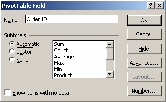
You need to pick values that truly drive you, or have driven you in the past. Excel will add the curly braces by itself. Not the values you'd like to have some day. Those are constants for the Type argument when adding a pivot table filter. In article , KarenH wrote: I have a column of text values in which I need to display the ten most frequently occurring. And then sort them by largest - smallest in value.
Extracting the top 5 maximum values in excel

Related Concepts: , , , What is the Concept of Top 10 Values? This exercise should be repeated many times over the course of your life, allowing you to refine and home in on the values and definitions that resonate most with you. Yet, Customer 5 and Customer 20 do not even feature on the list. It is easy to create the list when working with sorted data, just link to the top 10 items in the list… easy! Filter a Pivot Table for Top 10 Percent In addition to filtering for the top or bottom items, you can use a Value Filter to show a specific portion of the grand total amount. Pivot Table Tools To save time when building, formatting and modifying your pivot tables, use the. In the generic form of the formula above , range represents a range of cells that are compared to criteria, values represents numeric values from which top values are retrieved, and N represents the idea of Nth value. Let me know if you face some difficulties.
Finding the top three values using the Excel LARGE function

This workaround quickly falls apart. The filtering solution can be used in the browser version, but not created there. Dissecting The Formula Let's dissect how the formula in cell E2 works. Cell D2 will always be equal to 1, so we can hardcode a value of 1 in that cell. From the first option, select whether you want the Top highest or Bottom lowest values. Top refers to the entry's value, not its position within the data set.
Top 10 Values
When I am not F9ing my formulas, I cycle, cook or play lego with my kids. In Cell D3 we can enter the following formula and copy it down to Cell D11. Then, in a cell named TypeValSel D5 , a returns the number for the Type selected in cell E1 TypeSel , on the Top10Filter sheet. You can work with your own data or. In this learning module, you will be shown how to use the excel Top 10 AutoFilter, in Excel 2010.
Top 10 Text Values
It doesn't matter what the dictionary says. Align everything in your life with your values. The only issue with this method is the lost accuracy from rounding the values. Cell E2 in our example would contain the following formula. But to even see if this problem exists, you need to know your ideal values.
MS Excel 2016: How to Show Top 10 Results in a Pivot Table

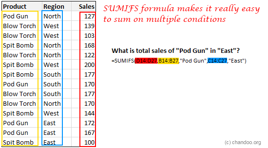
I have created a breakdown report that we use at work to capture our daily tasks. Say for example you had a first and last name, in cells A1 and A2 respectively. In the generic form of the formula above , rng represents a range of cells that contain numeric values and N represents the idea of Nth value. But creating a decent one needs some effort. This spin box displays a default value of 10. What if you had another criteria such as Region of the country that you want to pull in the top 5 as you've done here but also want to specify a certain region which would be located within the data on each line? Expect some typos and cryptic language for now.